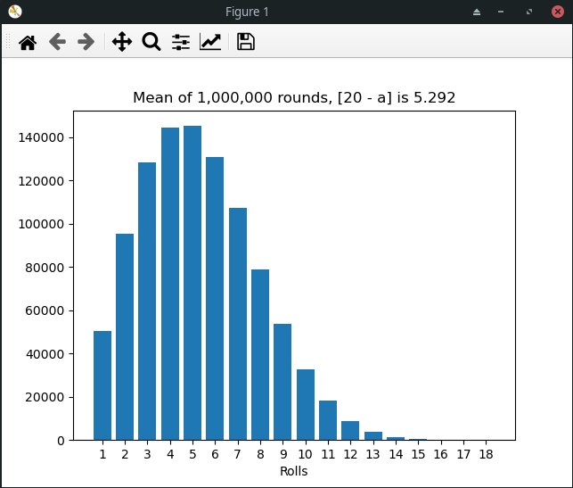
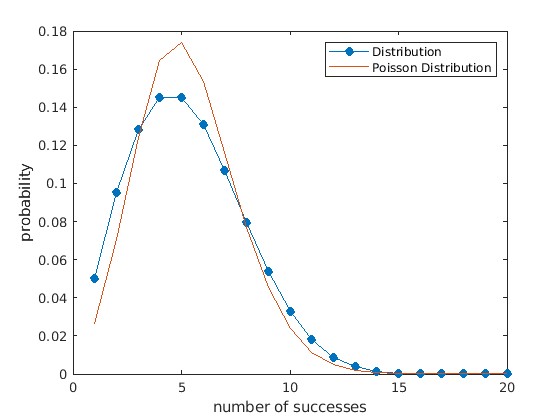
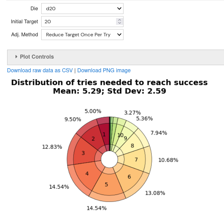
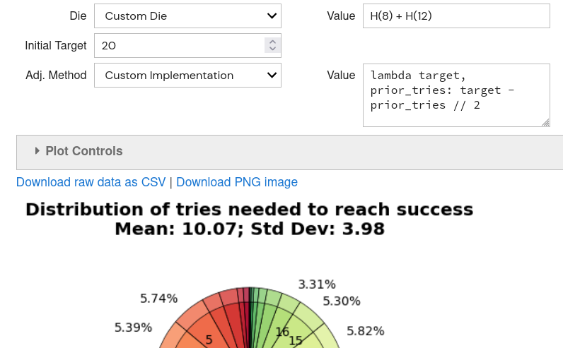
If I'm reading correctly, the fundamental prompt centers around the ability to (efficiently) iterate on variations of a game mechanic. Those more skilled than I am are better suited to derive a generalized formula mathematically, but I can at least provide some means for tinkering, in this case using dyce¹ for computation and anydyce² for rudimentary interaction.
You can try it out in your browser:  [source]

While admittedly a little clunky, the interface allows the user to select a die from the standard polygonal dice, define a target, and select an adjustment function from one of two predefined methods identified in the initial question. It also affords custom inputs for advanced users (more on this below).
Using dyce to Model the Mechanic
dyce uses discrete computation, meaning it achieves precision without randomized sampling. It doesn't do continuous distributions, but it will get you precise results, assuming it can adequately model the problem.
First Attempt - Naive (Non-Performant) Approach
When defining the mechanic in terms that dyce can understand, one might do something like the following:
from dyce import H
from dyce.evaluation import HResult, foreach

def degrading_target_nonperformant(
  die: H,
  initial_target: int,
  prior_tries: int = 0,
) -> H:
  adjusted_target = initial_target - prior_tries
  current_tries = prior_tries + 1

  def _callback(d_result: HResult):
    if d_result.outcome >= adjusted_target:
      return current_tries
    else:
      return degrading_target_nonperformant(d_result.h, initial_target, prior_tries=current_tries)

  return foreach(
    _callback,
    die,
    limit=-1,  # do not limit recursion
  )
While the above is technically accurate, branching at whether each outcome meets the threshold leads to performance of roughly O(n!). In practice, this will only work for small dice or small targets. A die of H(20) and target of 20 will take eons (maybe literally).
d20 with target 3 --> 343 µs ± 3.51 µs per loop (mean ± std. dev. of 7 runs, 1,000 loops each)
d20 with target 4 --> 1.09 ms ± 5.63 µs per loop (mean ± std. dev. of 7 runs, 1,000 loops each)
d20 with target 5 --> 4.32 ms ± 149 µs per loop (mean ± std. dev. of 7 runs, 100 loops each)
d20 with target 6 --> 20.8 ms ± 240 µs per loop (mean ± std. dev. of 7 runs, 10 loops each)
...
Second Attempt - Refined (Performant) Approach
The good news is that we can introduce a counting trick to make things easier on ourselves. Rather than branch on each outcome, we can branch on the likelihood of hitting a particular target:
def degrading_target_performant(
  die: H,
  initial_target: int,
  prior_tries: int = 0,
) -> H:
  adjusted_target = initial_target - prior_tries
  current_tries = prior_tries + 1
  succeeds_or_fails_at_adjusted_target_h = die.ge(adjusted_target)

  def _callback(ge_result: HResult):
    if ge_result.outcome == 1:
      return current_tries
    elif ge_result.outcome == 0:
      return degrading_target_performant(die, initial_target, proir_tries=current_tries)
    else:
      assert False, "should never be here"

  return foreach(
    _callback,
    succeeds_or_fails_at_adjusted_target_h,
    limit=-1,  # do not limit recursion
  )
This takes our branching factor from n (the number of sides of our die) to 2, which leads to a performance of O(n), which is totally reasonable.
d20 with target 3 --> 85.1 µs ± 685 ns per loop (mean ± std. dev. of 7 runs, 10,000 loops each)
d20 with target 6 --> 171 µs ± 756 ns per loop (mean ± std. dev. of 7 runs, 10,000 loops each)
d20 with target 9 --> 272 µs ± 2.17 µs per loop (mean ± std. dev. of 7 runs, 1,000 loops each)
d20 with target 12 --> 366 µs ± 2.84 µs per loop (mean ± std. dev. of 7 runs, 1,000 loops each)
d20 with target 15 --> 461 µs ± 2.22 µs per loop (mean ± std. dev. of 7 runs, 1,000 loops each)
d20 with target 18 --> 563 µs ± 4.93 µs per loop (mean ± std. dev. of 7 runs, 1,000 loops each)
...
This gives us what we want:
>>> d20 = H(20)
>>> h = degrading_target_performant(d20, 20)
>>> print(h.format(scaled=True))
avg |    5.29
std |    2.59
var |    6.68
  1 |   5.00% |#################
  2 |   9.50% |################################
  3 |  12.83% |############################################
  4 |  14.54% |##################################################
  5 |  14.54% |##################################################
  6 |  13.08% |############################################
  7 |  10.68% |####################################
  8 |   7.94% |###########################
  9 |   5.36% |##################
 10 |   3.27% |###########
 11 |   1.80% |######
 12 |   0.88% |###
 13 |   0.38% |#
 14 |   0.14% |
 15 |   0.05% |
 16 |   0.01% |
 17 |   0.00% |
 18 |   0.00% |
 19 |   0.00% |
 20 |   0.00% |
Improvement - Parameterized Adjusted Target Function
Now we can turn to enabling experimentation. We have already parameterized the die and target we're using. Astute coders will note that we can refactor the above to also parameterize the means by which we compute the adjusted target. The substantive source to our version can be found here.
Custom Inputs
For those familiar with Python and dyce, one can input one's own custom histogram for the die (e.g., 2 @ H(6) for 2d6) and one can even define one's own custom target adjustment function that takes two arguments (target and prior_tries) and returns the adjusted target. The custom function can either be defined as a lambda expression, or it can contain full-fledged Python code (so long as it defines or assigns a callable of the appropriate signature to the _ symbol).
For example, to see how the mechanic would work with a d8 plus a d12 and an adjustment function that reduces the target ever other try, one could use a custom die of H(8) + H(12) and a custom adjustment function of lambda target, prior_tries: target - prior_tries // 2, or, if one prefers, something like:
def my_adjustment_func(target: int, prior_tries: int) -> int:
  return target - prior_tries // 2

_ = my_adjustment_func  # <-- "export" the function by assigning it to the _ variable

One word of caution when experimenting with your own adjustment function: it must converge, meaning it must eventually result in a 100% chance of success (e.g., a target of the minimum value of the die range), or the computation will never finish. I'll leave it as an exercise to the reader to think about how one might go about introducing a safeguard. 😉
Parting Thoughts
I have never found a stand-alone mean to be a useful tool for evaluating a game mechanic. What one often really cares about is distributions. d20 and 4d4 both have the same means, but are very different animals. In game design, play-testing is essential, but a good visualization tool can help you eliminate a lot of junk before it even gets to the table. While probably a matter of taste, anydyce's "burst" graphs are my best attempt (so far) to get a "feel" for informing that process of elimination. I hope this helps in exploring your mechanic more thoroughly!
¹ dyce is my Python dice probability library.
² anydyce is my visualization layer for dyce meant as a rough stand-in for AnyDice.

